Part II · Candidate generation · chapter 8 of 19

Encoding objects: learned embeddings against content

A free embedding table is the most powerful model of an object that is possible at all. This whole chapter is about how nearly impossible it is to use that power, and about the one way out that works: constrain the model so that rare objects inherit knowledge from frequent ones. The key argument — «the tail of features is shorter and thicker than the tail of items» — is not asserted here but checked.

What to take away

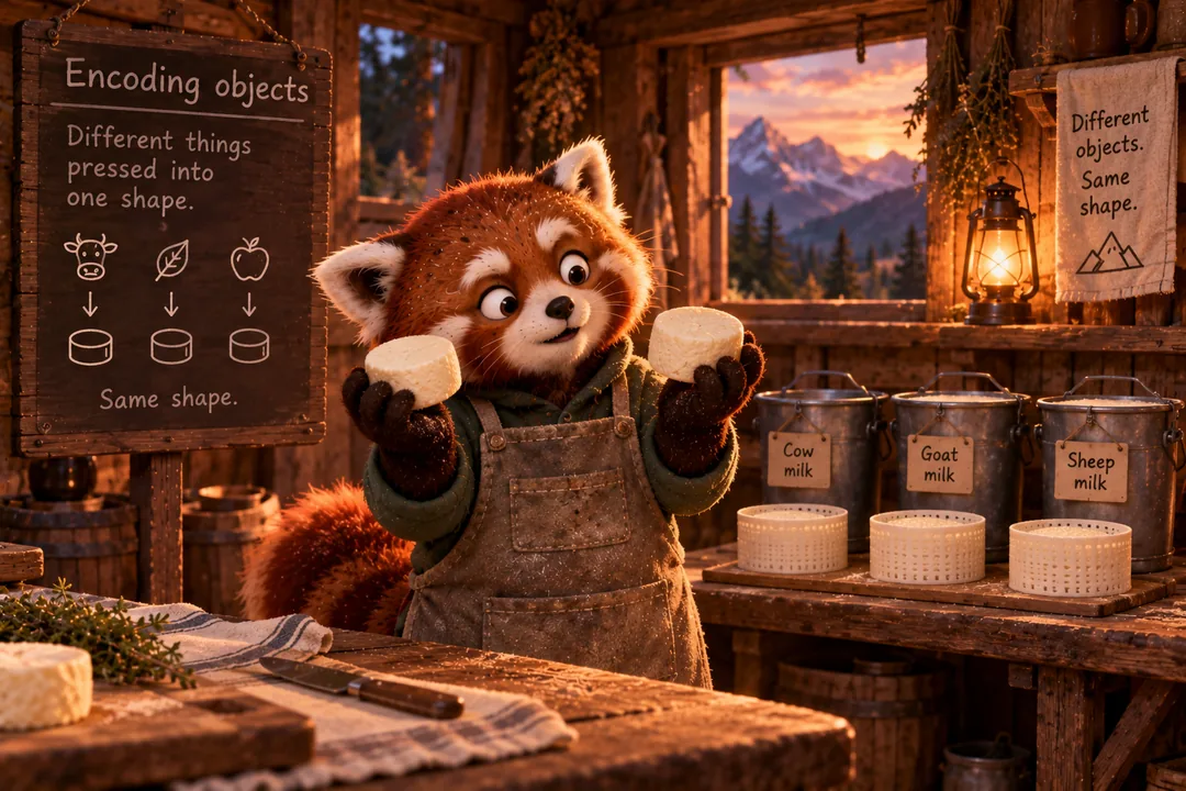
ID embeddings are the upper bound of expressiveness. Whatever a content encoder produces, the table can produce the same. The converse is false.
And that is exactly why they do not work on the tail. For 97.7% of items there are more free parameters than observations about them — the problem is underdetermined.
The tail of features really is shorter. Fewer than ten observations: 74.2% of items and 0.0% of features. The medians are 4.5 against 1275, a difference of 283 times.
Overfitting here is abrupt rather than gradual: quality grows through the first epoch and breaks off at the start of the second.

1. Learned embeddings

What «tied to an identifier» means

Literally: the embedding is fetched by the object's number from a table, like a value from a dictionary by its key.

$$ h(i) \;=\; E\bigl[\mathrm{id}(i)\bigr], \qquad E \in \mathbb{R}^{|\mathcal{I}| \times k} $$

The table $E$ is $|\mathcal{I}|$ rows of $k$ numbers, and row $j$ is trained only when item $j$ lands in a batch. The model receives no other information about the object: no title, no picture, no category. The only thing it knows is which row the object is in.

A check of understanding

Take two products with absolutely identical descriptions but different ids. Their vectors under ID embeddings will be in no way related — they were trained independently, and the coincidence of their content is simply unavailable to the model.

What is more: re-upload a product with a new id and everything accumulated about it is reset to zero.

The opposite approach is one where the vector is computed from features: $h(i) = f_\theta(\mathrm{features}(i))$. Here the id takes no part at all, and two identical products get identical vectors automatically.

Why this is the most powerful model of an object

A claim stronger than «it works well»

Every object has $k$ parameters of its own, tied to nothing else. So any arrangement of vectors is reachable: there is not a single constraint on where item $i$ ends up relative to item $j$. Taking $k = |\mathcal{I}|$, any similarity matrix can be reproduced exactly.

Hence a consequence: whatever a content encoder produces, the table can produce the same. The encoder's output is one particular assignment of vectors to objects, and the table accepts any assignment. The converse is false: the encoder is bound by features and has to give identical vectors to two items with identical descriptions, even when the data says they behave differently.

That is, ID embeddings have zero inductive bias. This is the upper bound of power — and at the same time the source of all the problems below: there is nothing to hold a model without constraints back from memorising noise.

A practical consequence worth remembering

On the head of the catalogue ID embeddings usually beat any content representation: they learn what is not in the features at all. Two outwardly identical products can convert differently because of the seller, the price, the reviews, the photograph — the table picks that up, an encoder over the title does not.

So in production ID features are almost never thrown out entirely. The final construction is nearly always hybrid, and the question is not «what instead of what» but «in what proportion».

2. Why that power cannot be used

All five problems grow from one root: a row of the table is trained only on the examples where that exact item occurred. There is little data per row, and there is nothing to link it to the rows of similar items.

How little «little» is

A catalogue of 10 M, a billion interactions, dimension 256, popularity following Zipf with $\alpha = 1$:

Observations about an item	Share of the catalogue	Their share of interactions
fewer than 10	40.1%	3.1%
fewer than 100	94.0%	16.9%
fewer than 256 (= the dimension)	97.7%	22.5%

The numbers are reproduced by the script _tools/tail_table.py in this repository.

The last row is the verdict: 97.7% of items have more free parameters than observations about them. For such a row the problem is underdetermined, and «training» turns into fitting a few points.

Drawback 1. Transductivity

The model applies only to the objects of the training set. A new item appears — and in the table there is either no row for it or a row from random initialisation that no gradient has ever touched. There is nowhere to take a value from: there is nothing to compute it out of, and the model does not accept features.

And a random vector in a trained space is not «neutral»: it will land randomly close to some cluster and get scores that look meaningful and are not.

The problem is wider than «a new product»: new users are the same thing from the other side of the matrix; changing an identifier resets everything accumulated; rare categories are formally not cold but with two or three observations behave exactly as if they were.

Drawback 2. Memorisation and a heavy tail

What memorisation is formally

Storing individual examples instead of deriving a general regularity. It is measured through the influence of an example: train two models — with it and without it — and compare the error on that example.

a small difference → the model generalised: there are similar examples in the data and the knowledge came from them;
a large difference → there are no similar ones, and the model simply memorised it.

Now apply this to an item that occurred once. Remove it and the error is enormous: we know nothing about it. Add it and there is still not enough data to understand who will like it. All the model can do is remember that it occurred for one particular user.

A conclusion worth remembering word for word

The heavy tail holds the items with few examples. We can memorise them, but it is hard to recommend them.

Memorising the tail is not harmful in itself — we are merely spending capacity on something not very useful. The harm starts when the same mechanism memorises noise: that is overfitting.

And telling an adequate rare example from noise is hard for a model: from the outside they look identical — one observation with no similar ones. Free embeddings meanwhile greatly increase the capacity for memorisation. Strong memorisation plus noisy data is guaranteed overfitting.

Drawback 3. Drift

Why a table cannot do «now»

The row $E[j]$ is updated every time the item lands in a batch, and the gradients from every episode add up into one vector. When training on shuffled data, an interaction from a year ago and one from yesterday contribute equally — what comes out is an averaged representation of the object over all time.

The problem is asymmetric: the head of the catalogue is updated constantly and drifts along with the data, the tail almost never is. The row of a rare item holds its state as of its last appearance in a batch, and that may have been a month ago.

Catastrophic forgetting

The obvious solution is to train chronologically and keep fine-tuning. But during fine-tuning the gradient arrives only for the items in the new window. The other rows stand still — while everything around them changes: user vectors are updated, the coordinate system shifts, the weights of the upper layers change.

A row placed correctly relative to the old space turns out to be placed randomly relative to the new one. The result is a trap: shuffled data gives an outdated average, chronological data gives a mismatch between the fresh part of the table and the stale one.

There is one radical way out: make the representation computed. Then updating the features automatically updates the vector, and no fine-tuning is required.

Drawback 4. Memory

The arithmetic that closes the question

Where tens of billions of embeddings come from: it is not only items. In an industrial model trainable vectors are created for everything categorical — the id of the item, the user, the author, the ad slot, the country, the device model — and also for cross features such as the pair «user × category». The number of rows multiplies rather than adds.

$$ 2\cdot10^{10} \times 256 \times 4\ \text{bytes} \;\approx\; \mathbf{20.5\ \text{TB}} $$

With Adam's moments (two tensors of the same size) — 61 TB. At dimension 4096, as is fashionable in LLMs — 328 TB of weights and nearly a petabyte together with the optimiser.

Recomputed by the script _tools/tail_table.py.

What that means in engineering terms

The table does not fit on a GPU — not on one, not on a node. So either sharding across devices, or storage in RAM and on parameter servers with the needed rows fetched per batch.
Training is bound by the network, not by computation. The model on top of the embeddings may be tiny; the bottleneck is moving rows between nodes. That inverts the usual optimisation: computing faster is pointless, you have to send less.
Most of those terabytes are the tail, which we are only memorising anyway. We pay memory for rows that bring no generalisation.

Drawback 5. Overfitting and the one-epoch phenomenon

What is actually observed

Quality grows gradually through the first epoch and falls sharply at the start of the second. Not a slow degradation but a break — and that is the difference from computer vision, where a model is trained for hundreds of epochs and overfitting sets in gradually.

The practical consequence in production: the best result is usually given by training for exactly one epoch. Many industrial pipelines are built that way — a single pass over the stream.

Three factors and a hypothesis about the cause

The effect is associated with the architecture (embedding + MLP), a fast-converging optimiser and feature sparsity. The last is the main one: the finer the granularity of a feature — and an item id is as fine as it gets — the stronger the effect.

The mechanism: write the representation of an example after the embedding layer as $\mathrm{EMB}(x)$. The joint distribution $\bigl(\mathrm{EMB}(x), y\bigr)$ is different for examples the model has already seen and for new ones: for the seen ones the embedding has had time to adapt to their label. On the second epoch every training example is a seen one, the MLP quickly adapts to exactly that distribution — and loses its applicability to new ones.

That is, the model overfits not to the examples in the usual sense but to an artefact of its own embedding table.

Why you cannot simply «reduce the sparsity»

The effect really does weaken and even disappear if rare values are filtered out or hashed into a smaller number of buckets. But it is honestly stated in the same place: this often leads to worse final quality.

The logic is familiar: rare features are at once the source of the overfitting and the source of exactly the signal ID embeddings were created for. Throwing out the tail removes the overfitting along with the usefulness.

Hence the whole programme of the second half of this chapter: not to throw out the tail and not to forbid memorisation, but to give the model a way to generalise between similar objects.

3. Inductive bias

Constraints on a model that increase its ability to generalise. We reduce the power, raise the bias and reduce the variance, lower memorisation — and with it the overfitting to noise.

The simplest example: a bag of words

Suppose the items are products with names. Tokenise the name, take trainable token embeddings, average them:

$$ h(i) = \frac{1}{|T_i|}\sum_{t \in T_i} e_t $$

What assumptions have we baked in? First: products with similar names have similar vectors. Second: word order does not matter.

The second assumption is false — «a case for an iPhone» and «an iPhone for a case» are not the same thing. But that is precisely the price of generalisation: the constraint is inexact, and in exchange a rare product gets a vector built from frequent tokens.

A check of intuition

Three models: (1) free embeddings, (2) an encoder over one feature, (3) an encoder over two. Where is the inductive bias larger?

The answer: 1 < 3 < 2. Free embeddings have the smallest bias — they are constrained by nothing. And a model with two features has more degrees of freedom than one with a single feature, so its bias is smaller than the second model's.

A useful rule: more features means less inductive bias, because the model can lean on a larger number of distinguishing signals and start «recognising» particular objects again.

4. Content encoding: checking the central argument

The argument for content is stated like this: the tail of features is shorter and thicker than the tail of items. It sounds like a metaphor, but it is a checkable claim.

Two tails side by side

A catalogue of 100 000 following Zipf with $\alpha = 1.2$, ten million interactions. Every item is described by six features from a vocabulary of 5 000 — that is, features are reused between items.

Fewer observations than	Share of items	Share of features
10	74.2%	0.0%
100	96.2%	0.1%
256 (= the dimension)	98.3%	3.7%

The numbers are reproduced by the script _tools/content_tail.py in this repository.

The median number of observations: 4.5 for an item, 1275 for a feature — 283 times more.

And the most telling line: the rarest item of the catalogue is expected to have 1.96 observations, while its six features have been seen 479, 6 088, 2 528 025, 536 660, 3 446 and 6 088 times. Nothing is known about the item itself, and everything is known about what it is made of.

Plus a saving in parameters

A free table is 100 000 rows, and 98.3% of them have fewer observations than the dimension. The content table is 5 000 rows, and only 3.7% are like that. Twenty times fewer parameters, and each of them trained on an incomparably larger volume.

That is the mechanism by which content pulls the tail up: a rare item is not trained on its own, it inherits knowledge from the frequent features it is assembled from.

What is paid for it

A ceiling on the head. Two products with identical descriptions get identical vectors, even when there is enough data to know that they convert differently.
The quality of the features becomes critical. Poor tokenisation or a thin taxonomy limits the model more than any architecture does.
More expensive at inference. The vector has to be computed rather than fetched. For items that is cured by precomputation, for user features not always.

So in production it is almost always a hybrid: the content part gives generalisation and cold start, the ID part picks up what is not in the features. The proportion is chosen by experiment.

5. Hashing: a compromise between the two

An intermediate technique that deserves a section of its own, because it is everywhere.

The idea and the price

Instead of a table «id → row» we take $h(\mathrm{id}) \bmod H$, where $H$ is fixed. The size of the table stops depending on the cardinality of the feature.

The price is collisions: several ids share one row and become indistinguishable to the model. The probability that a particular pair collides is $1/H$; with several independent hash functions, complete indistinguishability requires a collision under all of them, and the probability becomes a product.

And a second, less obvious gain: a new object is representable immediately. There is no need to wait for its id to enter a vocabulary and for the vocabulary to be rebuilt — the hash is computed at once. For a fast-changing catalogue that is not an optimisation but a necessary condition.

What to look for here

Reduce the size of the table: the share of items sharing a row with somebody grows faster than it seems — that is the birthday paradox.
Add a second hash function: the probability of complete indistinguishability falls as a product, while memory grows linearly. A favourable trade.
Watch who the collisions hurt: popular items suffer less, because they have enough data to «pull» a shared row towards themselves. It is the tail that pays for collisions again.

What to say in an interview: «Hashing trades memory for collisions and removes the dependence on cardinality. Several hash functions make complete indistinguishability a product of probabilities. And it makes a new object representable without rebuilding the vocabulary».

Interview questions

Why are ID embeddings called the most powerful model of an object?

Every object has $k$ parameters of its own, tied to nothing else, so any arrangement of vectors is reachable; at $k = |\mathcal{I}|$ any similarity matrix is reproduced.

Hence a consequence: whatever a content encoder produces, the table can produce the same — the encoder's output is one particular assignment, and the table accepts any. The converse is false: the encoder has to give identical vectors to objects with identical features.

That is, their inductive bias is zero. This is the upper bound of expressiveness and at the same time the cause of every problem: there is nothing to hold the model back from memorising noise.

Why do free embeddings work badly on the tail?

Because a row of the table is trained only on the examples containing that item, and there is nothing to link it to the rows of similar ones. The arithmetic: with a catalogue of 10 M, a billion interactions and dimension 256, 97.7% of items have more free parameters than observations about them.

For such a row the problem is underdetermined. All the model can do is memorise individual observations, and it is in no position to tell a rare but genuine signal from noise — from the outside they look identical.

What is the one-epoch phenomenon, and why can't you just reduce the sparsity?

Quality grows through the first epoch and falls sharply at the start of the second — a break rather than a gradual degradation, unlike computer vision. The practical consequence: the best result often comes from training for exactly one epoch, and industrial pipelines are built that way.

The hypothesised cause: the distribution $(\mathrm{EMB}(x), y)$ differs between seen and new examples, because for the seen ones the embedding has adapted to the label. On the second epoch the MLP adapts to precisely the distribution of the seen ones and loses its applicability to new ones. That is, the overfitting is to an artefact of the model's own table.

The sparsity can be reduced — filter out rare values or hash them into fewer buckets — and the effect really does weaken. But that often worsens the final quality: rare features are at once the source of the overfitting and the source of the signal they were introduced for.

Why does content encoding pull the tail up?

Because the tail of features is shorter and thicker than the tail of items, and that is checkable. On a catalogue of 100 thousand with six features from a vocabulary of 5 thousand: fewer than ten observations for 74.2% of items and for 0.0% of features. The medians are 4.5 for an item against 1275 for a feature, a difference of 283 times.

The mechanism is reuse: a rare item is assembled from frequent features. The rarest item of the catalogue is expected to have two observations, while its features have been seen between 479 and 2.5 million times. Nothing is known about the item itself, everything is known about what it is made of.

Plus the saving: 5 thousand rows instead of 100 thousand, and 3.7% of them have fewer observations than the dimension instead of 98.3%.

What is paid for moving to content features?

A ceiling on the head of the catalogue: two products with identical descriptions get identical vectors, even when there is enough data to know that they convert differently. ID embeddings pick that up, an encoder over features does not.

Plus the quality of the features becomes critical — poor tokenisation limits you more than any architecture — and the vector has to be computed rather than fetched, which is more expensive at inference.

So in production it is a hybrid: content gives generalisation and cold start, ID picks up what is not in the features. The question is not «what instead of what» but in what proportion.

What does the hashing trick give besides saving memory?

The main thing is that a new object is representable immediately. There is no waiting for the id to enter a vocabulary and for the vocabulary to be rebuilt: the hash is computed at once. For a fast-changing catalogue that is not an optimisation but a condition of the thing working.

The price is collisions: several ids share a row and become indistinguishable. Several independent hash functions make complete indistinguishability a product of probabilities while memory grows linearly — a favourable trade.

And an important detail: collisions hit the tail. A popular item has enough data to pull a shared row towards itself; a rare one does not.

One-screen cheat sheet

ID embedding

$h(i) = E[\mathrm{id}(i)]$. Zero inductive bias, the upper bound of power, zero generalisation between objects.

The arithmetic of the tail

97.7% of items have more parameters than observations. The problem is underdetermined.

Five drawbacks

Transductivity, memorisation, drift with forgetting, memory in terabytes, the break at the second epoch.

Two tails

Fewer than 10 observations: 74.2% of items and 0.0% of features. Medians 4.5 against 1275.

The price of content

A ceiling on the head, dependence on feature quality, costlier inference. Hence the hybrid.

Hashing

Memory for collisions plus instant representability of the new. Collisions hit the tail.

Primary sources

V. Feldman, C. Zhang. What Neural Networks Memorize and Why, NeurIPS 2020 — the definition of memorisation through the influence of an example and its connection with the long tail.
Z. Zhang, W. Wang et al. Towards Understanding the Overfitting Phenomenon of Deep Click-Through Rate Prediction Models, CIKM 2022 — one-epoch: the break at the start of the second epoch, three factors, a hypothesis about the cause.
K. Weinberger, A. Dasgupta et al. Feature Hashing for Large Scale Multitask Learning, ICML 2009 — the hashing trick and bounds on collisions.
B. Coleman, W.-C. Kang et al. Unified Embedding: Battle-Tested Feature Representations for Web-Scale ML Systems, NeurIPS 2023 — how this is done at industrial scale.
The numbers in this chapter: _tools/tail_table.py and _tools/content_tail.py in this repository.