
 RecSys
 Part II · Candidate generation · chapter 9 of 19
ANN, quantisation and semantic IDs
The vectors are trained — now they have to be searched. This is an engineering chapter and it closes candidate generation: why exhaustive search does not fit the budget, how approximate search is built, and which knob in it trades recall for speed. At the end, a technique that replaces a vector with a short hierarchical code and turns search into generation.
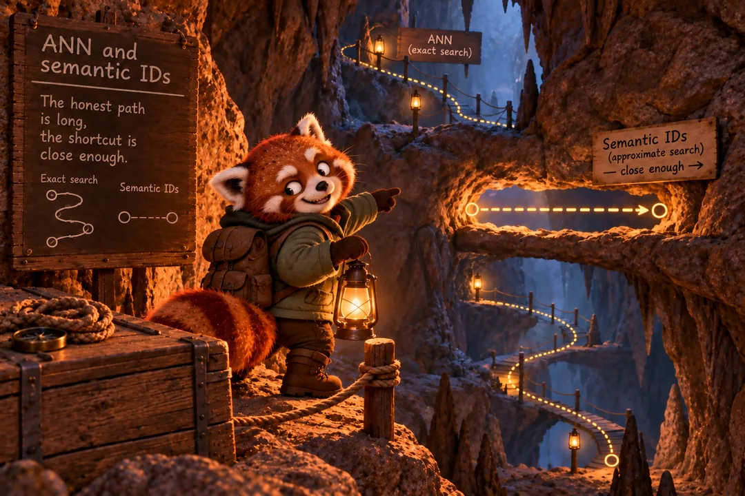
- ANN is approximate by definition. It does not «sometimes make mistakes» — it trades recall for speed, and the knob of that trade turns at runtime without rebuilding the index.
- Exhaustive search: 5.1 billion operations per request with a catalogue of 10 M and dimension 256. Of the order of 100 ms against a budget of 10.
- Quantisation compresses 32-fold — 32 bytes per vector instead of 1024 — at the price of a noticeable error in the distance.
- A semantic ID of six levels of 256 is 6 bytes instead of 1024. And three levels already suffice to address an item in a catalogue of 10 M; the rest refine.
1. Why exact search will not do
The task after training two towers is to find the \(k\) items with the largest inner product. This is MIPS, maximum inner product search.
$$ \operatorname{top-}k(u) \;=\; \operatorname*{arg\,max}_{i \in \mathcal{I}}{}^{(k)}\; \langle p_u, q_i\rangle $$Naively this is \(O(|\mathcal{I}| \cdot d)\) per request. With a catalogue of 10 M and dimension 256:
- 5.1 billion operations for a single request;
- about 100 ms at 50 GFLOPS — an order of magnitude more than the retrieval budget;
- 10.2 GB of memory for the index in float32.
The numbers are reproduced by the script _tools/ann_demo.py in this repository.
And that is for one request. A gap of an order of magnitude is not closed by constants — a different data structure is needed.
An important distinction interviewers like. With cosine similarity the norm \(\lVert q_i\rVert\) cancels; with an inner product it does not.
So MIPS systematically prefers items with a large norm, and the norm grows with popularity during training. This is a popularity bias built into the geometry itself rather than into the data.
In practice: the index has to be built for the measure the model optimises. The options are to normalise the embeddings and work with cosine, to build an index with an inner-product metric, or to reduce MIPS to ordinary neighbour search by adding a coordinate.
2. HNSW: how approximate search is built
Hierarchical Navigable Small World is the most widespread structure for ANN. Conceptually it is a skip list generalised to a metric space: several layers, each denser than the one above, and on every layer the graph has the small-world property — between any two points there is a short path.
Building. Points are added one at a time. For each of them a maximum level is sampled from a geometric distribution with \(\lambda = 1/M\) — that is, exponential thinning, with about \(M\) times fewer points at each next level. The point automatically enters every layer below its maximum. Then a bounded traversal with a queue of size efConstruction, and the \(M\) nearest points found are connected by edges.
Searching. We start at the top layer, where there are few points. On each layer we walk along the neighbours while the distance to the query greedily decreases, then drop a level. On the bottom layer there is a bounded traversal with the efSearch queue, maintaining a heap of the top \(k\) along the way.
The size of the queue on the bottom layer is the «recall against latency» trade on an already-built index. It turns at runtime and requires no rebuild.
Hence an important practice: keep one index and tune ef to the current load. That also gives you a ready mechanism for controlled degradation — under a spike, lower ef and return slightly less complete results instead of returning a five-hundred.
- Memory. The graph stores up to \(M\) edges per node per layer, so HNSW is noticeably hungrier than quantised indexes. That is exactly why IVF-PQ and ScaNN exist.
- Updates. Deletion is done by marking, and the index degrades over time, requiring a rebuild. For a fast-changing catalogue that is an engineering pain of its own — and one of the reasons an ANN can lose to simpler sources in a news feed.
- Set
efSearch = 1: the traversal visits a handful of nodes and finds a small fraction of the true neighbours. An ANN does not guarantee the right answer — it is approximate by definition. - Pull
efSearchup: Recall@10 reaches 1.00, but the number of visited nodes triples. The right-hand curve shows both quantities at once — that is the Pareto front of «recall against latency». - Further on the curve flattens: recall is already one while the traversal keeps getting more expensive. You should work at the knee, not to the right of it.
What to say in an interview: «HNSW is a multi-layer graph with exponential thinning, search in \(O(\log N)\). efSearch trades recall for latency at runtime with no rebuild. The weak spots are memory for the edges and degradation under deletions».
3. Quantisation: paying accuracy for memory
The second family of indexes saves not traversal time but memory and the cost of a distance.
A vector is cut into \(m\) subvectors, a codebook of \(2^b\) centroids is trained for each piece, and the vector is stored as \(m\) centroid numbers instead of \(d\) numbers.
$$ q_i \;\approx\; \bigl[\,c^{(1)}_{k_1},\; c^{(2)}_{k_2},\; \ldots,\; c^{(m)}_{k_m}\,\bigr], \qquad k_j \in \{1 \ldots 2^{b}\} $$The distance is computed over the codebooks through a precomputed table: for a query the distances to all centroids are computed once, after which the distance to any vector is \(m\) additions.
A catalogue of 10 M, dimension 256, \(m = 32\) subvectors of 8 bits:
| originally | 10.2 GB | 1024 bytes per vector |
| after PQ | 0.32 GB plus 0.3 MB of codebooks | 32 bytes per vector |
| compression | 32-fold | |
The numbers are reproduced by the script _tools/ann_demo.py.
The price is honest and worth naming: the average error per coordinate after quantisation is about 0.43 with a coordinate spread of 1.0. That is, distances are computed noticeably approximately, and recall falls.
The standard way out is a two-phase search: select several hundred candidates using the compressed index, then recompute exact distances from the original vectors for those alone. Memory is saved on the whole catalogue, accuracy is restored on a small top.
A separate line worth knowing about: if the catalogue fits in GPU memory, exhaustive search can turn out faster than approximate search on a CPU. Matrix multiplication is exactly the operation a GPU is built for.
The gain is not only speed. Exact search removes three problems at once: no loss of recall, no index rebuild on updates, and the score need not be an inner product — which means two towers stop being mandatory and a more expressive similarity function can be computed.
The limitation is simple: the catalogue has to fit. For tens of millions of items at a modest dimension that is already realistic.
4. Semantic IDs: a vector becomes a code
A different approach to the same problem. Instead of searching by vector, let us replace the vector with a short hierarchical code.
We encode the vector sequentially: the first codebook approximates the vector itself, the second approximates the residual after the first approximation, the third the residual after the second, and so on.
$$ r_0 = q_i, \qquad k_\ell = \arg\min_j \lVert r_{\ell-1} - c^{(\ell)}_j \rVert, \qquad r_\ell = r_{\ell-1} - c^{(\ell)}_{k_\ell} $$The item turns into a tuple \((k_1, k_2, \ldots, k_L)\). The key difference from product quantization: the code comes out hierarchical. The first level sets a coarse region, each next one refines it.
A typical configuration is 6 levels of 256 values:
| addressable combinations | \(256^6 \approx 2.8 \cdot 10^{14}\) |
| length of the code | 48 bits = 6 bytes |
| against a float32 vector(256) | 1024 bytes |
| compression | 171-fold |
The numbers are reproduced by the script _tools/ann_demo.py.
The headroom in the address space for a catalogue of 10 M is seven orders of magnitude. So collisions, where they occur, arise not from a shortage of space but because two items really did land in the same cell by meaning.
With a catalogue of 10 M:
| Levels of code | Groups | Items per group |
|---|---|---|
| 1 | 256 | ≈ 39 062 |
| 2 | 65 536 | ≈ 153 |
| 3 | 16 777 216 | fewer than one |
The numbers are reproduced by the script _tools/ann_demo.py.
Three levels are already enough to address a particular item. The rest refine rather than distinguish — and that is not redundancy but the property the whole thing is done for.
Because items close in meaning get a shared prefix of the code. A new item landing in the same semantic region inherits the prefix — and a model that has never seen it already knows the main thing about it. This is the same technique as content encoding in the previous chapter: a rare object is assembled from frequent pieces.
If an item is a sequence of six tokens, then recommendation becomes a task of generating a sequence: the model predicts the code token by token, the way a language model predicts words.
What that changes:
- The index disappears. No ANN, no rebuilding, no trade of recall against latency — the model simply produces a code.
- The score stops being an inner product. The two-tower constraint is lifted: autoregression sees the tokens already generated.
- A problem of its own appears: the model can generate a code that corresponds to no item. Cured by constrained decoding over a prefix tree of existing codes.
This is one of the directions the field is moving in. It is still worth judging with restraint: the public results are encouraging, but few have reached the scale of a feed with tens of millions of items.
- Add levels of code and watch the reconstruction error: the first gives a coarse approximation, each next one shaves off the residual. The curve flattens quickly.
- Reduce the size of the codebook: the error grows but the code is shorter. That is the same «memory against accuracy» trade as in PQ.
- Compare with product quantization at an equal number of bits: in RQ the code is hierarchical, in PQ the pieces are independent — and no shared prefix arises for similar items.
What to say in an interview: «A semantic ID is a hierarchical code from residual quantisation. It gives hundredfold compression and a shared prefix for similar items, which is where cold start and generative retrieval come from. The price is a loss of accuracy and the risk of generating a code that does not exist».
5. What to choose
| Approach | When | What we pay |
|---|---|---|
| HNSW | a catalogue up to tens of millions, high recall needed, moderate updates | memory for the graph, degradation under deletions |
| IVF-PQ and relatives | the catalogue does not fit in memory in its original form | a noticeable loss of accuracy, a two-phase search is required |
| Exhaustive search on a GPU | the catalogue fits in GPU memory | the cost of the hardware; in exchange, freedom in the choice of similarity measure |
| Semantic IDs | cold start and compactness are needed and there is capacity for research | a loss of accuracy, the risk of invalid codes, the maturity of the approach |
And a general rule worth keeping in mind: choosing an index is not choosing an algorithm but choosing a point on the curve of «recall against latency against memory». Comparing options makes sense only with two of the three fixed.
Interview questions
Why can't you simply scan all the vectors?
The arithmetic does not add up. With a catalogue of 10 M and dimension 256 that is 5.1 billion operations per request — of the order of 100 ms at 50 GFLOPS, while the retrieval budget is usually 10 ms. A gap of an order of magnitude is not closed by constants.
Plus memory: 10.2 GB in float32 for the vectors alone.
A caveat: if the catalogue fits in GPU memory, exhaustive search can turn out faster than approximate search on a CPU, and then it is preferable — no loss of recall, no index rebuild, and the score need not be an inner product.
How does MIPS differ from nearest-neighbour search?
With cosine the norm of the vector cancels; with an inner product it does not. So MIPS systematically prefers items with a large norm, and the norm grows with popularity during training. The result is a popularity bias built into the geometry rather than into the data.
The practical consequence: the index has to be built for the measure the model optimises. Either normalise the embeddings and work with cosine, or take an index with an inner-product metric, or reduce MIPS to ordinary neighbour search by adding an extra coordinate.
How is HNSW built and what is efSearch?
A multi-layer graph — essentially a skip list generalised to a metric space. A point's level is sampled from a geometric distribution, so each next layer holds about M times fewer points. The search starts at the top, where there are few points, greedily descends along edges and drops a layer. The expected complexity is \(O(\log N)\).
efSearch is the size of the queue on the bottom layer, that is, the «recall against latency» knob on an already-built index. It changes at runtime with no rebuild, which is also why it serves as a mechanism of controlled degradation under load.
The weak spots: memory for the edges (up to M per node per layer) and degradation under deletions, which are done by marking and require periodic rebuilding.
What does product quantization give and what is paid for it?
A vector is cut into m subvectors, each encoded by a centroid number from its own codebook. At 256 dimensions with 32 subvectors of 8 bits a vector takes 32 bytes instead of 1024 — 32-fold compression, and a catalogue of 10 M shrinks from 10.2 GB to 0.32 GB.
Plus distances are computed faster: for a query the distances to all centroids are computed once, after which the distance to any vector is m table additions.
The payment is accuracy: the average error per coordinate is about 0.43 with a spread of 1.0. So a two-phase search is used — select hundreds of candidates on the compressed index, then recompute exact distances for those alone.
What are semantic IDs and what are they for?
A hierarchical code produced by residual quantisation: the first codebook approximates the vector, the second the residual, the third the residual of the residual. The item becomes a tuple of several tokens.
The arithmetic: 6 levels of 256 give \(2.8 \cdot 10^{14}\) combinations at a code length of 6 bytes against 1024 for a float32 vector — 171-fold compression. With a catalogue of 10 M, three levels already suffice to address an item; the rest refine.
But the point is not the compression, it is the hierarchy: items close in meaning get a shared prefix. A new item inherits the prefix of its region, and a model that has never seen it already knows the main thing about it. This is the same mechanism as content features — a rare object assembled from frequent pieces.
What is generative retrieval and what is its risk?
If an item is a sequence of tokens, recommendation becomes generation: the model predicts the code token by token, the way a language model predicts words. The index disappears entirely: no ANN, no rebuilding, no trade of recall against latency.
The two-tower constraint is lifted at the same time — the score stops being an inner product, because autoregression sees the tokens already generated.
The risk is specific: the model can generate a code that corresponds to no existing item. Cured by constrained decoding over a prefix tree of valid codes. And the approach is worth judging with restraint — few have taken it to the scale of tens of millions of items.
One-screen cheat sheet
Why ANN
5.1 billion operations and 100 ms per request at 10 M × 256. The budget is 10 ms.
MIPS ≠ NN
The norm does not cancel and grows with popularity. Build the index for the model's metric.
HNSW
Layers thinned M-fold, search in \(O(\log N)\). efSearch is the recall knob at runtime.
PQ
32 bytes instead of 1024, 32× compression, error 0.43 per coordinate. Hence the two-phase search.
Semantic ID
6 levels × 256 = 6 bytes, 171× compression. Three levels suffice to address, the rest refine.
The choice
Not a choice of algorithm but a point on the recall–latency–memory curve. Fix two of the three.
Primary sources
- Y. Malkov, D. Yashunin. Efficient and Robust Approximate Nearest Neighbor Search Using Hierarchical Navigable Small World Graphs, 2016 — the original work on HNSW.
- H. Jégou, M. Douze, C. Schmid. Product Quantization for Nearest Neighbor Search, TPAMI 2011.
- R. Guo, P. Sun et al. Accelerating Large-Scale Inference with Anisotropic Vector Quantization, ICML 2020 — ScaNN and quantisation sharpened for MIPS.
- S. Rajput, N. Mehta et al. Recommender Systems with Generative Retrieval, NeurIPS 2023 — semantic IDs and generative retrieval.
- The numbers in this chapter:
_tools/ann_demo.pyin this repository.